5.3 Gaussian Elimination

Systems of linear equations can be solved by placing the coefficients in a matrix, reducing the matrix to row-echelon form, and performing back substitution from the bottom up. The basis of this is a theorem attributed to Gauss.

Theorem 5.2 The following operations can be applied to a linear system without changing the solution set.

multiply both sides of an equation by a non-zero constant
exchange one equation with another
sum or subtract an equation with (possibly the multiple) of another

It is possible to apply these rules to the matrix of coefficients to produce a new matrix in which the leading non-zero element in each row is 1, and in which the element below a leading 1 is zero. Such a matrix is said to be in row-echelon form. Then new equations can be recovered from the new matrix. Finally, back substitution is performed to yield a solution.

Let's try this with the system

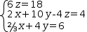(6⋅z=18, 2⋅x+10⋅y-4⋅z=4, 2/3⋅x+4⋅y=6)ℓ.

(1)

Converted to matrix form ^[1], this is

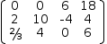[(0, 0, 6, 18), (2, 10, -4, 4), (2/3, 4, 0, 6)].

Myron always sorts the columns in ascending order of variable name so in this matrix the columns represent coefficients

y and

z with the constant in the last column.

Another way of looking at this matrix is as an expression that concatenates two matrices.

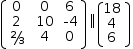[(0, 0, 6), (2, 10, -4), (2/3, 4, 0)]‖[(, 18), (, 4), (, 6)].

The matrix corresponding to variable coefficients is the left operand and the column matrix on the right corresponds to the constants. Matrices are often combined like this in order to perform coordinated elementary row operations on the individual matrices. A combined matrix is sometimes call an augmented matrix. The left-hand portion is sometimes called the unaugmented matrix.

Suitable application of Gauss' rules in a process called Gaussian elimination can reduce the matrix to row-echelon form, which is

[(1, 6, 0, 9), (0, 1, 2, 7), (0, 0, 1, 3)].

(2)

Note the 1's along the diagonal and the zeroes below the diagonal. This matrix agrees with Definition 5.4.

Definition 5.3 A pivot element is the leading non-zero element in a row of a matrix.

Definition 5.4 A matrix is in row-echelon form if

rows with at least one non-zero element are above rows consisting of all zero elements
For each row, the pivot element is always to the right of the pivot element in the row above

Matrix (2) is a representation of the system of linear equations ^[2]

(x_1+6⋅x_2=9, x_2+2⋅x_3=7, x_3=3)ℓ,

which is not quite in form of a solution.

To get from the row-echelon form to a final solution, the equations are worked from last to first. The last equation is usually in the form 1⋅x_i=b. For this matrix, the last equation is x_3=3. Working from the second-last to the first, isolate the left side and substitute in the right side. That is, isolate x_2 in x_2+2⋅x_3=7 ^[3], substitute x_3 ^[4] and simplify to x_2=1. Then isolate, substitute and simplify x_1+6⋅x_2=9 to get x_1=3.